Calculating entropy from costmap history
Background
As part of my ongoing research in the Building Wide Intelligence Project I have now begun to tackle a new problem: learning behavioral properties of obstacles from histories of costmaps. This essentially boils down to using histories of laser readings in order to classify obstacles as either static or dynamic (or more fine grained representations of dynamic). This could be provide a large improvement to our current infrastructure which only uses the laser readings to detect an obstacle. With our current approach, a wall, a human, a chair, and a trashcan will all appear the same to the robot and as such will be treated the same. However, it is clear that walls and humans do not behave in the same manner; a wall will remain in its location for the duration of its lifespan, whereas a human is a very dynamic obstacle. A human can and will move within short spans of time. My goal is to be able to learn these behavior properties using the histories of laser readings. My goal is to have the robot analyze how the costmaps (occupancy grids generated based on laser readings) change over time, in order to extrapolate and classify the obstacle types. I am working on this research under the advise of Dr. Jivko Sinapov in Dr. Peter Stone’s lab.
Costmaps
There isn’t much in the existing literature about using costmaps to learn behavior properties so I figured I should start collecting data to see what type of information I would have available to work with.
Our robots use ROS and are running the latest version of our codebase (which is entirely open source).
The portion of the current system infrastructure which is of interest is the global and local costmaps. The global costmap is updated on latching and contains a timestamp, information about the dimensions of the map, and an integer (8 bit integers) array which is a 2D representation of the cost map where each entry is the probability of an obstacle being there. The probabilities range from 0-100, with the exception of -1 which represents an unknown.
This occupancy grid is used by the navigator infrastructure to localize and to plan accordingly.
The current system does not keep any history of costmaps; it simply uses the latest one.
In addition to the global costmap, the robots also have a notion of a local costmap. This is the constantly updated from the laser readings and published at a frequency of 4Hz.
The local costmap only represents a small area around the robot within laser range, and is thus used to update the global costmap by replacing that chunk in the global costmap with the local costmap.
Collecting the costmaps
In order to capture the costmaps I decided to use our in-house bwi_logging tool to record ROS messages, which I upgraded to be able to handle arbitrary experimental topics. I then used our new uploading infrastructure so that costmaps could be automatically collected.
Experiment
As an experiment I had the robot autonomously navigating the corridors of our research lab while recording all the costmaps updates.
I recorded data for a total of 92 minutes which contained 1 global costmap and 17794 costmap updates. Uncompressed the data is 348mb but luckily it compresses well so the final file is only 23mb.
Once I had the data I wrote a program which used the rosbag interface to read the recorded messages and apply the patches at whatever interval I need. For the experiment I had it apply every single patch and save only the initial and final patched global maps.
The original map was 
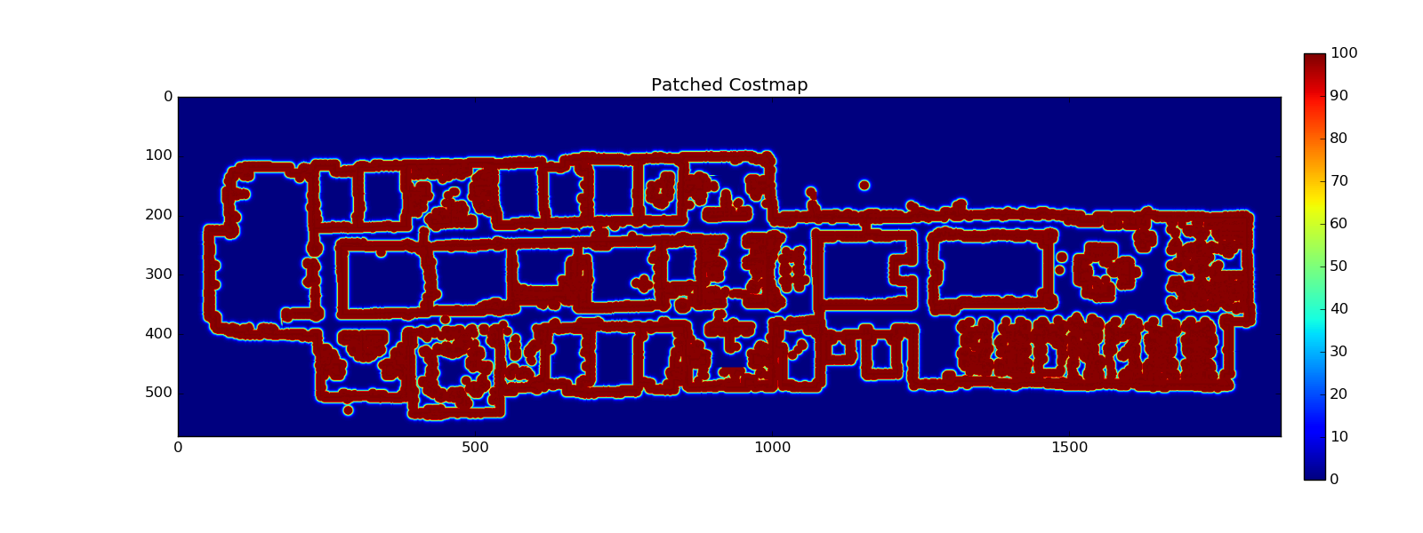
After applying all patches the final map was 
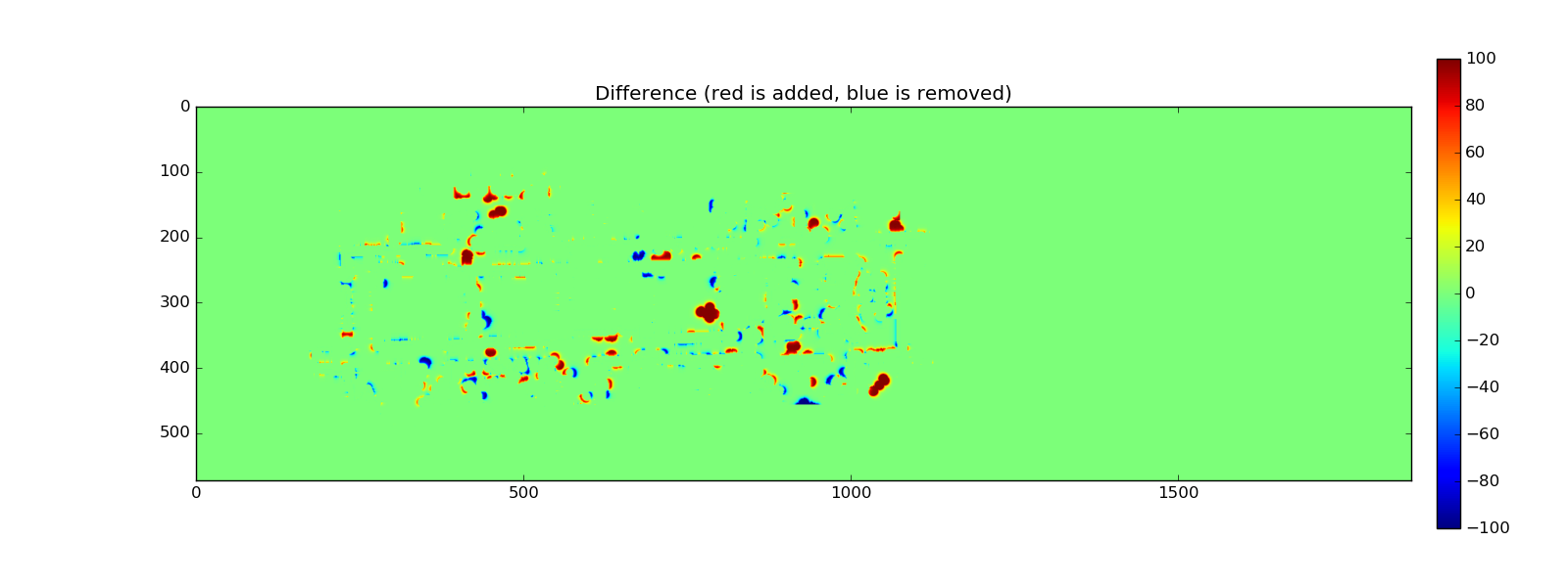
The differences are subtle when displayed side-by-side, but when
calculated they are clear 
This was an enlightening result because it gave me confidence that I might actually be able to learn something useful from these maps.
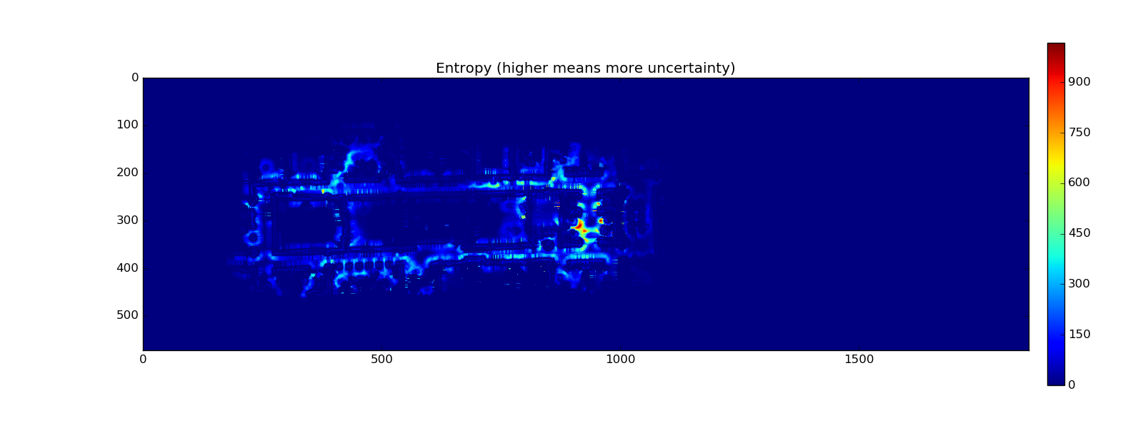
After talking with my research advisor he suggested I try to calculate the Shannon
entropy of the map to see what the highest entropy regions of the map are. Calculating
the entropy was as simple as keeping track which parts of the map change the most, so
whenever I apply the patches I keep track of areas that changed with the patch. This enabled
me to generate the following entropy heatmap 
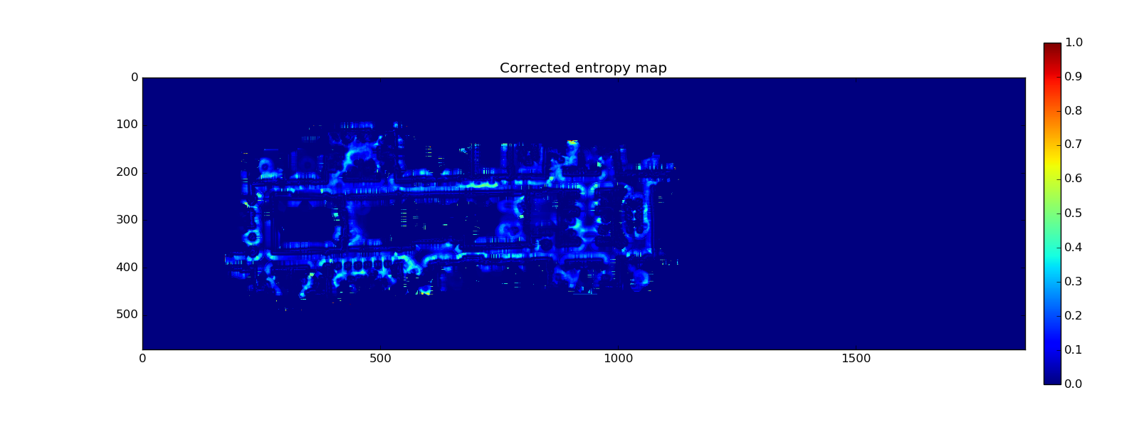
However, I soon realized that the calculation is unfairly biased against areas that the robot
did not visit often, since there would be less updates. So I normalized the data
by dividing the number of times an area changed by the number of times the robot actually
visited (and gained information from) that area. This method generated the following entropy map

This was an exciting result because it agrees with the areas that I would have imagined to have the highest entropy, such as the hallways, PhD cubicle area, and Dr. Stone’s office.
Next Steps
These maps show that there is definitely new information that can be learned from the histories of costmaps. Although they are not classifying obstacles yet, they can provide useful information. As such, the obvious next steps are how this information can be used to improve the robots. Three possible venues are localization, navigation, and planning. In terms of localization, the maps could be used to make better predictions and better probability models for the Monte Carlo particle filter localizer. For navigation these maps could be useful in case the robot encounters an obstacle. For example, if it is in a high entropy area it could decide to wait some time to see if the obstacle will move before giving up and trying to find a new path. And finally for planning, it might be useful to add the entropy maps as another cost layer, such that the planner will try to avoid high entropy areas.
Source Code
All the source code is currently available in my branch of the experimental source code on github